Introduction
This project was done as a part of the Data Science Retreat batch 6.
The original competition ran during the dates below.
Started: 9:22 am, Monday 13 December 2010 UTC
Ended: 10:00 pm, Sunday 20 February 2011 UTC (69 total days)
We however, completed our approach in a 3 day period.
Here we will describe our approach to creating a model.
The first problem we encountered with this dataset was that each row, which corresponded to each individual grant application, would have multiple columns to list aspects within a variable. For example, there was room for 15 people for each project, with each person being randomly allocated to either person 1 or person 2 columns in each row.
This was an issue, as a model would be unable to find trends in data if variables were split across columns. So to combat this we decided to create two smaller models to sum up the information contained within each person and their team. The first being the people model and the second being the team model.
Cleaning the Data
The original dataset from the University of Melbourne is formated quite ugly. There are 249 features, mainly because for every person working on a project there are 15 features describing this person and the maximium team size is 15 people. So 225 of the 249 features describe the people who created the application. As many application were created by teams much smaller than 15 people, most of the columns are filled very scarcely.
These 225 features were handled in the People and the Team Model, so the cleaning_all.r file just takes care of the first 24 features.
The date column was properly formated and these new features were derived from it: Weekday, Month, Day and Month, Day of Month and Season.
As there was a significant amount of missing values in the dataset, we had to find way to deal with them.
For the feature Contract Value Band, which is a factrorial variable classifying the contract value into 14 levels, we filled the missing data with random samples from an empirical distribution of the existing data.
For the columns Grant Category Code and Sponsor Code, which are factorial variables as well, we were able to use a more accurate model. As both variables are significantly correlated with the Contract Value Band, we could use this information to create conditional empirical distributions for Grant Category Code and Sponsor Code depending on the Contract Value Bandof the respective application.
Each application has up to 5 RFCD Codes, which describe the university departments working on this project and up to 5 socioeconomic objectives in the SEO Code columns. For each of these ten columns there is an additional column showing the percentage of the project related to the respective department or socioeconomic objectve. As the majority of the applications have a maximum of two departments and SEOs, most of these features are empty. To be able to use this part of the data, we created columns for each possible department and socioeconomic objective, stating respected percentage. This method allows all parts to be displayed individually. instead of checking five different columns to see if the project is related to a certain department, you have to check just one.
After the cleaning, the data was split into a training, a testing and a validation set.
Splitting
Because of the test data available lacked the Grant.Status field, i.e. the target we want to predict, we arrange our labeled data (training dataset) in the following way: in the first round,we take data from group 1 (see Figure 1) for training, and data from group 2 for validation (parameter tuning). After we achieved one model we were confident on it, we move to the second round, where we use data from group 1 and group 2 for training (keeping the same parameters learned) and used data from group 3 for testing. The predictions obtained in this group 3, are the results presented in the Results section.
You can find the exact Grant IDs used to do the splitting in the following files:
- testing_ids.txt
- training2_ids.txt
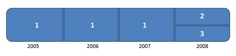
Figure 1. Splitting data.
Data Analysis
The applicants' ability to write a good application might influence the probability of success significantly, so we needed to find a way to measure this talent. The measure for this talent was called People Score. As there were more than 3000 different people working on the applications in the dataset, we decided analyze the people score in a different model. The result of this model is a table of the unique IDs with their respective People Score.
As can be seen in Figure 2, the Team Model uses the output from the People Model and the 225 features describing the persons working on the application from the original dataset. From this information several new featured are designed and given as input to the final model.
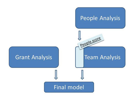
Figure 2. Overview of our analysis on the presented features.
People Analysis
The people model takes the data output from cleaning_all.R and uses it to build a table that has one row for each person ID/project combination, alongside each individual variable that correspond to each person.
This is built from a for loop that takes each set of variables from each person on each row and then gives it its own row on a new table, alongside whether the application succeeded or failed.
This table is then cleaned to make it ready for logistic regression, through methods such as changing NAs to seperate factors, changing non factor variables to factor variables and removing NA people ID rows.
Initially, the table contained too large an amount of factors, with each person ID and all possible departments and faculties. We reduced the amount of factors by lumping the least important factors together.
This was done as the model function used had hard limits on the number of factors that could be used as inputs and those factor levels that had the least people involved were deemed to contain the least predictive information, making a good target for simplifying the table.
This data is then saved in the data folder as peopleTable.RData
This is then used by the people_model.R script to build a glm() binomial logistic regression model using each persons variables to predict their grant application status success. The coefficients from this model associated with each person ID is then used as the 'people score' in the Team Model.
Team Analysis
This part of the data consist on evaluate how strong a team is. Along the time, the researchers move from one department to another, ask for different grants forming subgroups within the same department, so we need to evaluate a team as a combination of researchers that actually applied to an specific grant.
The 'people score' obtained from the previous step include negative values, positive values, and comprises a non-defined range. Hence the first step is to normalize them in the range [0,1]. In order to build the feature called "People.score" in this part, we sum the normalized score of all the participants that applied for a specific grant. We also computed, "Avg.People.score" to ensure that teams with one top researcher does not be outnumbered by big teams with lower profiles.
Other features included where "Dif.countries" that takes into account how many different countries can be found in a team, "Departments" the ammount of different departmenst involved (as they will have different viewpoints that can better tackle unseen problems) and "Perc_non_australian" to take into account that many times a fraction of the grants are kept for integrate inmigrants and people from abroad in the society.
This was a non exhaustive list of the features. More information can be found in the python code.
Grant Analysis
The final model predicts if a grant application will be accepted or not. A random forest with 3000 trees is used for this classification. The input variables are the combination of the output of the Team Model with the cleaned and rebuilt data from the University of Melbourne.
In total the model uses 65 features, 14 of them are taken from the output of the Team Model. The rest of the features are either taken from the original competition dataset or directly engineered from it.
The number of variables randomly sampled as candidates at each split was optimized, and the optimum value found was 7.
Computational time was about one minute.
Results
The model produces an Area Under the Curve (AUC) of 0.914 as can be seen in Figure 3. This result would have placed us on rank 78 on the Kaggle Competition leaderboard (Figure 4). However as the competition was already over, we were not able to test our model on the official testing data. Instead we cut our testing set from the training data. If we had been able to train this model on the full training data, we might have been able to achieve an even better result.
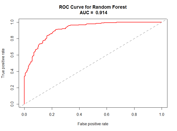
Figure 3. ROC plot and AUC = 0.914.
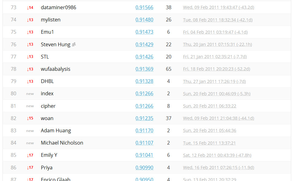
Figure 4. Kaggle's public leaderboard for this challenge.
The following table (Table 1) shows the confusion matrix with the real values as rows and the predicted values as columns.
| Granted | Not Granted | |
| Granted | 482 | 22 |
| Not Granted | 384 | 603 |
Table 1. Confusion matrix.
The model is quite good at finding the applications which will eventually get granted, even though it missclassifies some of the application which did not receive funding.
The most important features were:
- Number of unsuccessful applications of Team members
- Number of successful applications of Team members
- Sponsor of the Grant
- Day of Month
- Month
- Contract Value Band
- Grant Category Code
All these variables are intuitively related to the success of an application,except for Day of Month and Month. A possible explanation for the high importance of these features is, that for many sponsors the probability of granting funding decreases to zero after reaching their budget. This makes it less likely for an application to be successful later in the months.
Similar reasoning might explain the importance of the month of the application. At certain times of the year, their maybe varying funding budgets aswell as a varying number of competing applications.